Adversarial Autoencoders (with Pytorch)

Introduction

“Most of human and animal learning is unsupervised learning. If intelligence was a cake, unsupervised learning would be the cake [base], supervised learning would be the icing on the cake, and reinforcement learning would be the cherry on the cake. We know how to make the icing and the cherry, but we don’t know how to make the cake.”

Director of AI Research at Facebook, Professor Yann LeCunn repeatedly mentions this analogy at his talks. By unsupervised learning, he refers to the “ability of a machine to model the environment, predict possible futures and understand how the world works by observing it and acting in it.”

Deep generative models are one of the techniques that attempt to solve the problem of unsupervised learning in machine learning. In this framework, a machine learning system is required to discover hidden structure within unlabelled data. Deep generative models have many widespread applications, density estimation, image/audio denoising, compression, scene understanding, representation learning and semi-supervised classification amongst many others.

Variational Autoencoders (VAEs) allow us to formalize this problem in the framework of probabilistic graphical models where we are maximizing a lower bound on the log likelihood of the data. In this post we will look at a recently developed architecture, Adversarial Autoencoders, which are inspired in VAEs, but give us more flexibility in how we map our data into a latent dimension (if this is not clear as of now, don’t worry, we will revisit this idea along the post). One of the most interesting ideas about Adversarial Autoencoders is how to impose a prior distribution to the output of a neural network by using adversarial learning.

If you want to get your hands into the Pytorch code, feel free to visit the GitHub repo. Along the post we will cover some background on denoising autoencoders and Variational Autoencoders first to then jump to Adversarial Autoencoders, a Pytorch implementation, the training procedure followed and some experiments regarding disentanglement and semi-supervised learning using the MNIST dataset.

Background

Denoising Autoencoders (dAE)

The simplest version of an autoencoder is one in which we train a network to reconstruct its input. In other words, we would like the network to somehow learn the identity function $f(x) = x$. For this problem not to be trivial, we impose the condition to the network to go through an intermediate layer (latent space) whose dimensionality is much lower than the dimensionality of the input. With this bottleneck condition, the network has to compress the input information. The network is therefore divided in two pieces, the encoder receives the input and creates a latent or hidden representation of it, and the decoder takes this intermediate representation and tries to reconstruct the input. The loss of an autoencoder is called reconstruction loss, and can be defined simply as the squared error between the input and generated samples:

$$L_R (x, x’) = ||x - x’||^2$$

Another widely used reconstruction loss for the case when the input is normalized to be in the range $[0,1]^N$ is the cross-entropy loss.

Variational Autoencoders (VAE)

Variational autoencoders impose a second constraint on how to construct the hidden representation. Now the latent code has a prior distribution defined by design $p(x)$. In other words, the encoder can not use the entire latent space freely but has to restrict the hidden codes produced to be likely under this prior distribution $p(x)$. For isntance, if the prior distribution on the latent code is a Gaussian distribution with mean 0 and standard deviation 1, then generating a latent code with value 1000 should be really unlikely.

This can be seen as a second type of regularization on the amount of information that can be stored in the latent code. The benefit of this relies on the fact that now we can use the system as a generative model. To create a new sample that comes from the data distribution $p(x)$, we just have to sample from $p(z)$ and run this sample through the decoder to reconstruct a new image. If this condition is not imposed, then the latent code can be distributed among the latent space freely and therefore is not possible to sample a valid latent code to produce an output in a straightforward manner.

In order to enforce this property a second term is added to the loss function in the form of a Kullback-Liebler (KL) divergence between the distribution created by the encoder and the prior distribution. Since VAE is based in a probabilistic interpretation, the reconstruction loss used is the cross-entropy loss mentioned earlier. Putting this together we have,

$$L(x, x’) = L_R (x, x’) + KL(q(z|x)||p(z))$$ or $$L(x, x’) = - \sum _{k=1} ^{N} x _k \ log(x’ _k) + (1- x _k) \ log(1 - x’ _k) + KL(q(z|x)|| p(z))$$

Where $q(z|x)$ is the encoder of our network and $p(z)$ is the prior distribution imposed on the latent code. Now this architecture can be jointly trained using backpropagation.

Adversarial Autoencoders (AAE)

AAE as Generative Model

One of the main drawbacks of variational autoencoders is that the integral of the KL divergence term does not have a closed form analytical solution except for a handful of distributions. Furthermore, it is not straightforward to use discrete distributions for the latent code $z$. This is because backpropagation through discrete variables is generally not possible, making the model difficult to train efficiently. One approach to do this in the VAE setting was introduced here.

Adversarial autoencoders avoid using the KL divergence altogether by using adversarial learning. In this architecture, a new network is trained to discriminatively predict whether a sample comes from the hidden code of the autoencoder or from the prior distribution $p(z)$ determined by the user. The loss of the encoder is now composed by the reconstruction loss plus the loss given by the discriminator network.

The image shows schematically how AAEs work when we use a Gaussian prior for the latent code (although the approach is generic and can use any distribution). The top row is equivalent to an autoencoder. First a sample $z$ is drawn according to the generator network $q(z|x)$, that sample is then sent to the decoder which generates $x’$ from $z$. The reconstruction loss is computed between $x$ and $x’$ and the gradient is backpropagated through $p$ and $q$ accordingly and its weights are updated.

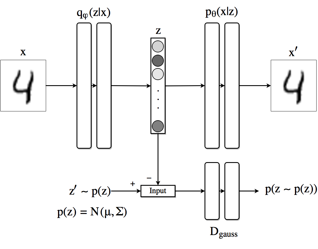
Figure 1. Basic architecture of an AAE. Top row is an autoencoder while the bottom row is an adversarial network which forces the output to the encoder to follow the distribution $p(z)$.

On the adversarial regularization part the discriminator recieves $z$ distributed as $q(z|x)$ and $z’$ sampled from the true prior $p(z)$ and assigns a probability to each of coming from $p(z)$. The loss incurred is backpropagated through the discriminator to update its weights. Then the process is repeated and the generator updates its parameters.

We can now use the loss incurred by the generator of the adversarial network (which is the encoder of the autoencoder) instead of a KL divergence for it to learn how to produce samples according to the distribution $p(z)$. This modification allows us to use a broader set of distributions as priors for the latent code.

The loss of the discriminator is

$$L_D = - \frac{1}{m} \sum _{k=1} ^m \ log(D(z’)) + \ log(1 - D(z))$$ (Plot)

where $m$ is the minibatch size, $z$ is generated by the encoder and $z’$ is a sample from the true prior.

For the adversarial generator we have

$$L_G = - \frac{1}{m} \sum _{k=1} ^m log(D(z))$$ (Plot)

By looking at the equations and the plots you should convince yourself that the loss defined this way will enforce the discriminator to be able to recognize fake samples while will push the generator to fool the discriminator.

Network definition

Before getting into the training procedure used for this model, we look at how to implement what we have up to now in Pytorch. For the encoder, decoder and discriminator networks we will use simple feed forward neural networks with three 1000 hidden state layers with ReLU nonlinear functions and dropout with probability 0.2.

#Encoder
class Q_net(nn.Module):
    def __init__(self):
        super(Q_net, self).__init__()
        self.lin1 = nn.Linear(X_dim, N)
        self.lin2 = nn.Linear(N, N)
        self.lin3gauss = nn.Linear(N, z_dim)
    def forward(self, x):
        x = F.droppout(self.lin1(x), p=0.25, training=self.training)
        x = F.relu(x)
        x = F.droppout(self.lin2(x), p=0.25, training=self.training)
        x = F.relu(x)
        xgauss = self.lin3gauss(x)
        return xgauss

# Decoder
class P_net(nn.Module):
    def __init__(self):
        super(P_net, self).__init__()
        self.lin1 = nn.Linear(z_dim, N)
        self.lin2 = nn.Linear(N, N)
        self.lin3 = nn.Linear(N, X_dim)
    def forward(self, x):
        x = self.lin1(x)
        x = F.dropout(x, p=0.25, training=self.training)
        x = F.relu(x)
        x = self.lin2(x)
        x = F.dropout(x, p=0.25, training=self.training)
        x = self.lin3(x)
        return F.sigmoid(x)

# Discriminator
class D_net_gauss(nn.Module):
    def __init__(self):
        super(D_net_gauss, self).__init__()
        self.lin1 = nn.Linear(z_dim, N)
        self.lin2 = nn.Linear(N, N)
        self.lin3 = nn.Linear(N, 1)
    def forward(self, x):
        x = F.dropout(self.lin1(x), p=0.2, training=self.training)
        x = F.relu(x)
        x = F.dropout(self.lin2(x), p=0.2, training=self.training)
        x = F.relu(x)
        return F.sigmoid(self.lin3(x))

Some things to note from this definitions. First, since the output of the encoder has to follow a Gaussian distribution, we do not use any nonlinearities at its last layer. The output of the decoder has a sigmoid nonlinearity, this is because we are using the inputs normalized in a way in which their values are within 0 and 1. The output of the discriminator network is just one number between 0 and 1 representing the probability of the input coming from the true prior distribution.

Once the networks classes are defined, we create an instance of each one and define the optimizers to be used. In order to have independence in the optimization procedure for the encoder (which is as well the generator of the adversarial network) we define two optimizers for this part of the network as follows:

torch.manual_seed(10)
Q, P = Q_net() = Q_net(), P_net(0)     # Encoder/Decoder
D_gauss = D_net_gauss()                # Discriminator adversarial
if torch.cuda.is_available():
    Q = Q.cuda()
    P = P.cuda()
    D_cat = D_gauss.cuda()
    D_gauss = D_net_gauss().cuda()
# Set learning rates
gen_lr, reg_lr = 0.0006, 0.0008
# Set optimizators
P_decoder = optim.Adam(P.parameters(), lr=gen_lr)
Q_encoder = optim.Adam(Q.parameters(), lr=gen_lr)
Q_generator = optim.Adam(Q.parameters(), lr=reg_lr)
D_gauss_solver = optim.Adam(D_gauss.parameters(), lr=reg_lr)

Training procedure

The training procedure for this architecture for each minibatch is performed as follows:

1) Do a forward path through the encoder/decoder part, compute the reconstruction loss and update the parameteres of the encoder Q and decoder P networks.

    z_sample = Q(X)
    X_sample = P(z_sample)
    recon_loss = F.binary_cross_entropy(X_sample + TINY,
                                        X.resize(train_batch_size, X_dim) + TINY)
    recon_loss.backward()
    P_decoder.step()
    Q_encoder.step()

2) Create a latent representation z = Q(x) and take a sample z’ from the prior p(z), run each one through the discriminator and compute the score assigned to each (D(z) and D(z’)).

    Q.eval()
    z_real_gauss = Variable(torch.randn(train_batch_size, z_dim) * 5)   # Sample from N(0,5)
    if torch.cuda.is_available():
        z_real_gauss = z_real_gauss.cuda()
    z_fake_gauss = Q(X)

3) Compute the loss in the discriminator as and backpropagate it through the discriminator network to update its weights. In code,

    # Compute discriminator outputs and loss
    D_real_gauss, D_fake_gauss = D_gauss(z_real_gauss), D_gauss(z_fake_gauss)
    D_loss_gauss = -torch.mean(torch.log(D_real_gauss + TINY) + torch.log(1 - D_fake_gauss + TINY))
    D_loss.backward()       # Backpropagate loss
    D_gauss_solver.step()   # Apply optimization step

4) Compute the loss of the generator network and update Q network accordingly.

# Generator
Q.train()   # Back to use dropout
z_fake_gauss = Q(X)
D_fake_gauss = D_gauss(z_fake_gauss)

G_loss = -torch.mean(torch.log(D_fake_gauss + TINY))
G_loss.backward()
Q_generator.step()

Generating images

Now we attempt to visualize at how the AAE encodes images into a 2-D Gaussian latent representation with standard deviation 5. For this we first train the model with a 2-D hidden state. Then we generate uniform points on this latent space from (-10,-10) (upper left corner) to (10,10) (bottom right corner) and run them to through the decoder network.

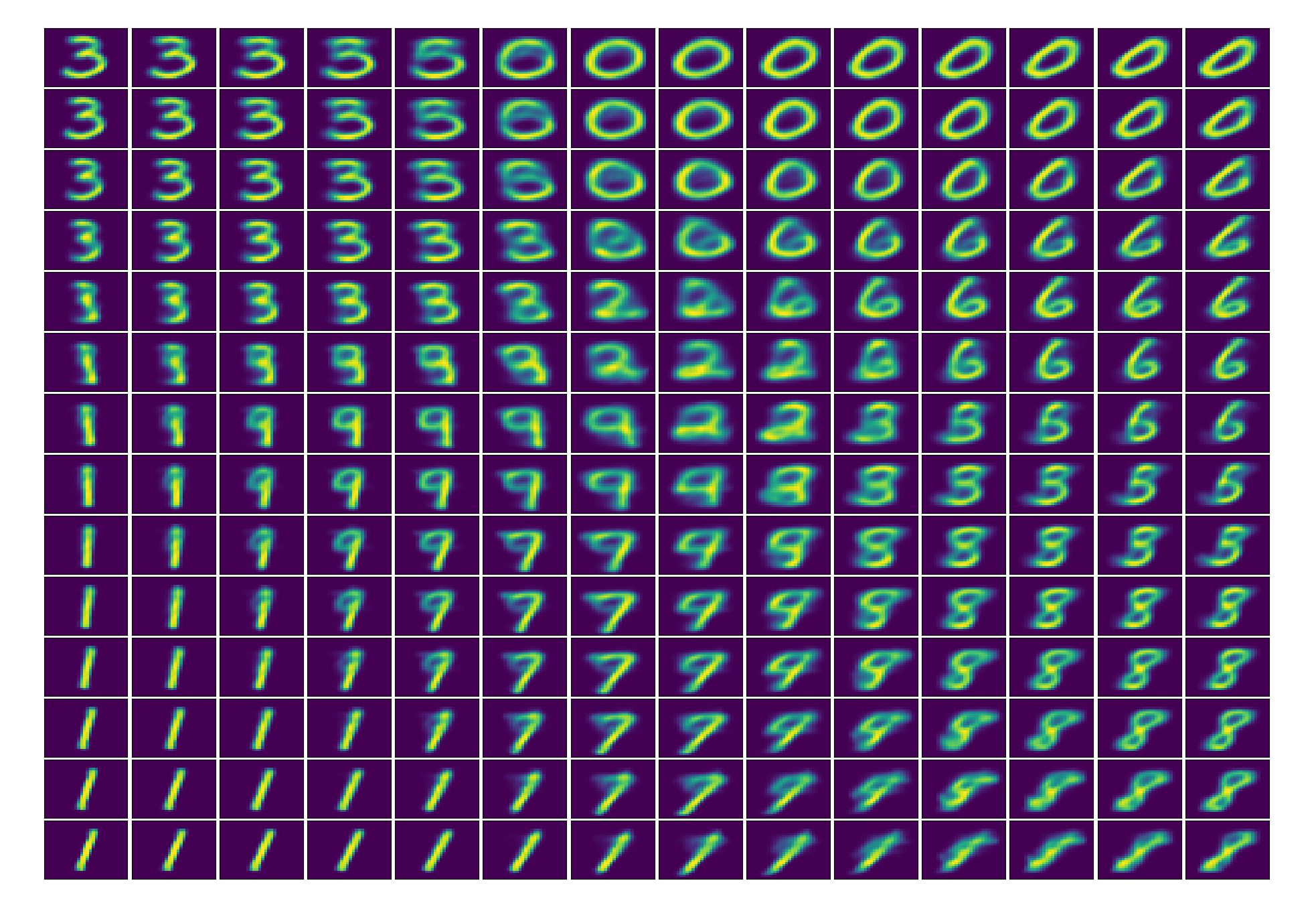
Latent space. Image reconstructions while exploring the 2D latent space uniformly from -10 to 10 in both the $x$ and $y$ axes.

AAE to learn disentangled representations

An ideal intermediate representation of the data would be one that captures the underlying causal factors of variation that generated the observed data. Yoshua Bengio and his colleagues note in this paper that “we would like our representations to disentangle the factors of variation. Different explanatory factors of the data tend to change independently of each other in the input distribution”. They also mention “that the most robust approach to feature learning is to disentangle as many factors as possible, discarding as little information about the data as is practical”.

In the case of MNIST data (which is a large dataset of handwritten digits), we can define two underlying causal factors, on the one hand, we have the number being generated, and on the other one the style or way of writing it.

Supervised approach

In this part, we go one step further than the previous architecture and try to impose certain structure in the latent code $z$. Particularly we want the architecture to be able to separate the class information from the trace style in a fully supervised scenario. To do so, we extend the previous architecture to the one in the figure below. We split the latent dimension in two parts: the first one $z$ is analogous as the one we had in the previous example; the second part of the hidden code is now a one-hot vector $y$ indicating the identity of the number being fed to the autoencoder.

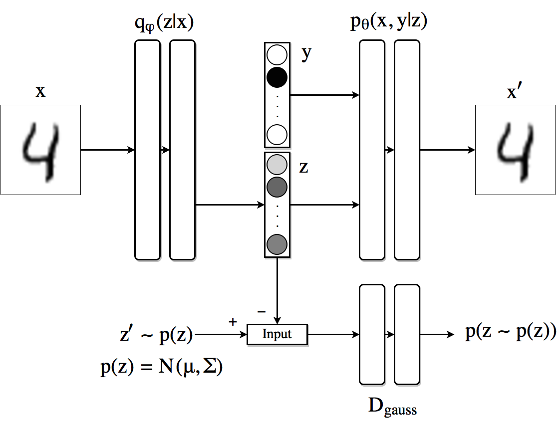
Supervised Adversarial Autoencoder architecture.

In this setting, the decoder uses the one-hot vector $y$ and the hidden code $z$ to reconstruct the original image. The encoder is left with the task of encoding the style information in $z$. In the image below we can see the result of training this architecture with 10,000 labeled MNIST samples. The figure shows the reconstructed images in which, for each row, the hidden code $z$ is fixed to a particular value and the class label $y$ ranges from 0 to 9. Effectively the style is maintained across the columns.

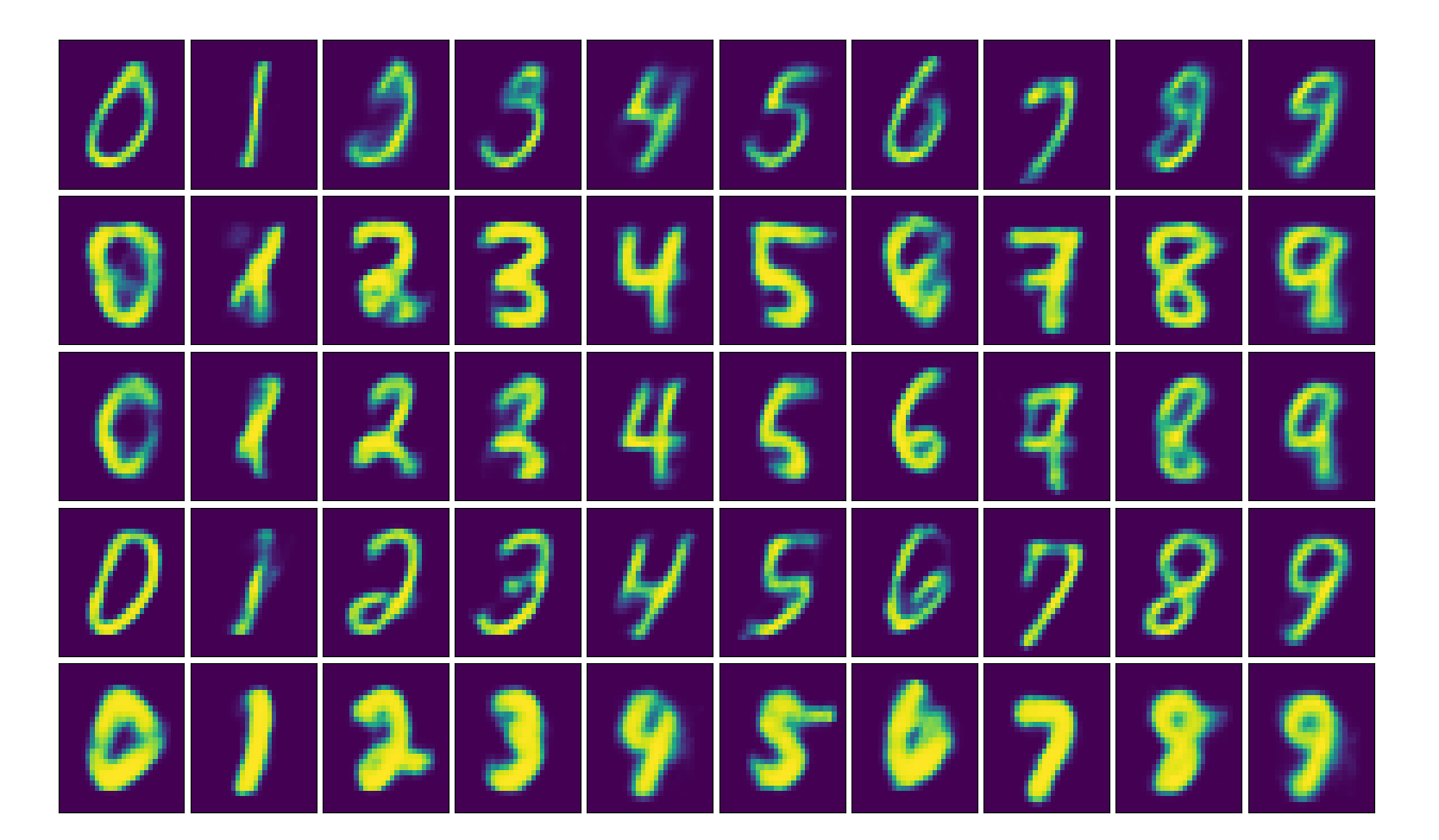
Image reconstruction by exploring the latent code $y$ while keeping $z$ fixed from left to right.

##### Semi-supervised approach As our last experiment we look an alternative to obtain similar disentanglement results for the case in which we have only few samples of labeled information. We can modify the previous architecture so that the AAE produces a latent code composed by the concatenation of a vector $y$ indicating the class or label (using a Softmax) and a continuous latent variable $z$ (using a linear layer). Since we want the vector $y$ to behave as a one-hot vector, we impose it to follow a Categorical distribution by using a second adversarial network with discriminator $D_{cat}$. The encoder now is $q(z, y|x)$. The decoder uses both the class label and the continuous hidden code to reconstruct the image.

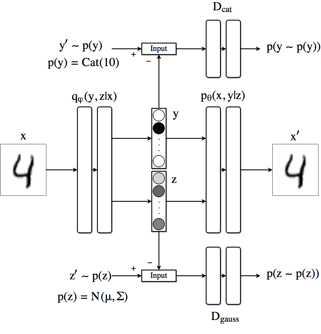
Semi-supervised Adeversarial Autoencoder architecture.

The unlabeled data contributes to the training procedure by improving the way the encoder creates the hidden code based on the reconstruction loss and improving the generator and discriminator networks for which no labeled information is needed.

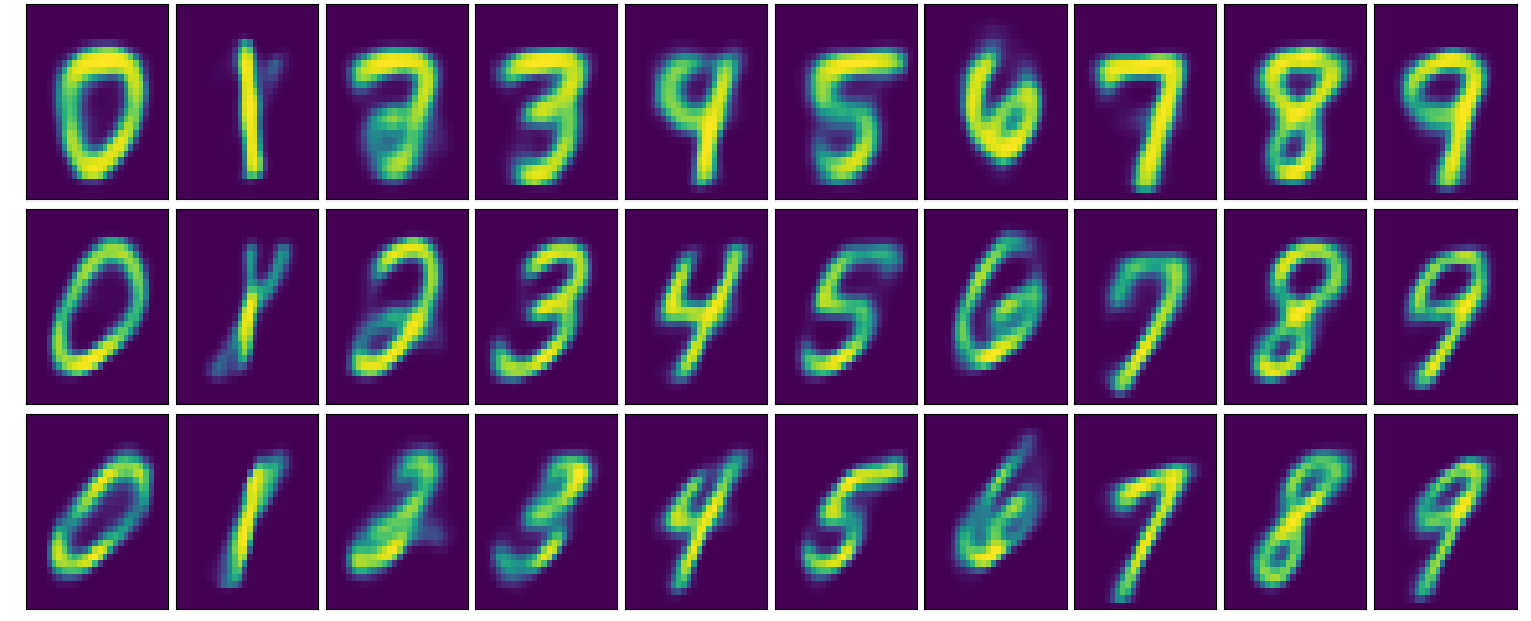
Disentanglement with semi supervised approach.

It is worth noticing that now, not only we can generate images with fewer labeled information, but also we can classify the images for which we do not have labels by looking at the latent code $y$ and picking the one with the highest value. With the current setting, the classification loss is about 3% using 100 labeled samples and 47,000 unlabeled ones.

On GPU training

Lastly, we do a short comparison in training time for this last algorithm in two different GPUs and CPU in Paperspace platform. Even though this architecture is not highly complicated and it is composed by few linear layers, the improvement in training time is enormous when making use of GPU acceleration. 500 epochs training time goes down from almost 4 hours in CPU to around 9 minutes using the Nvidia Quadro M4000 and further down to 6 minutes in the Nvidia Quadro P5000.

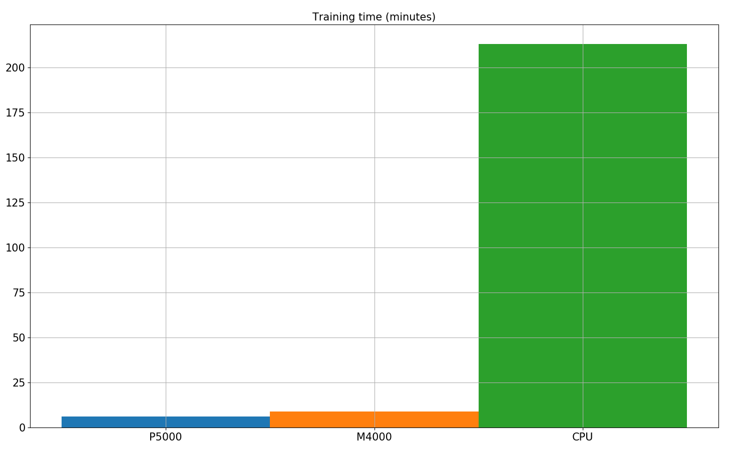
Training time with and without GPU acceleration

More material

• What is a variational autoencoder (Tutorial)
• Auto-encoding Variational Bayes (original paper)
• Adversarial Autoencoders (original paper)
• Building Machines that Imagine and Reason: Principles and Applications of Deep Generative Models